import pandas as pd
import optuna
from sklearn.svm import SVC
import geopandas as gpd
import pycountry
from sklearn.model_selection import cross_val_score
from sklearn.neural_network import MLPClassifier
from sklearn.metrics import accuracy_score
from sklearn.ensemble import RandomForestClassifier, VotingClassifier
import plotly.express as px
from sklearn.model_selection import train_test_split
from xgboost import XGBClassifier
from matplotlib.colors import ListedColormap
import numpy as np
import matplotlib.pyplot as plt
import seaborn as sns


pd.plotting.register_matplotlib_converters()
%matplotlib inlineDatathon Project-UCI MSF Team
Members: Songhan Hu, Jiaye Liu, Luoning Zhang Dataset: Market Analysis in Dublin
Objectives
1. Understanding the Guest’s Portrait
- Distribution of min and max price they’re searching
- How early do they book the Aribnb check in date (searching) - searching date
- Nights staying
- origin country
- room type
- neigborhood
2. Understanding the Demand of the Guests
- What types of guests tend to inquire/be accepted/successfully book/sucessfully check in?
- Why did some guests search but didn’t book?
Method
Business Model: Funnel Model Training a LGBM Model after comparing multiple ML models Visualization
Data Cleaning and Pre-processing
df1 = pd.read_csv('contacts.tsv', delimiter='\t',parse_dates=['ds_checkin','ds_checkout'])
df2 = pd.read_csv('searches.tsv', delimiter='\t',parse_dates=['ds','ds_checkin','ds_checkout'],)
df_s = df2.copy()
df_s['filter_room_types'] = df_s['filter_room_types'].apply(lambda x: [room.strip() for room in x.split(',')] if isinstance(x, str) else ['unknown'])
df_s['filter_neighborhoods'] = df_s['filter_neighborhoods'].apply(lambda x: [neighborhood.strip() for neighborhood in x.split(',')] if isinstance(x, str) else ['unknown'])
df_s['filter_room_types'] = df_s['filter_room_types'].apply(lambda x: set(x))
df_s['filter_neighborhoods'] = df_s['filter_neighborhoods'].apply(lambda x: set(x))
df_s['num_room_types'] = df_s['filter_room_types'].apply(lambda x: 0 if x == {'unknown'} else len(x))
df_s['day_diff'] = (df_s['ds_checkin'] - df_s['ds']).dt.days
df_s['num_neighborhoods'] = df_s['filter_neighborhoods'].apply(lambda x: 0 if x == {'unknown'} else len(x))
for i in df_s.index:
df_s.at[i, 'filter_room_types'] = [item for item in df_s.at[i, 'filter_room_types'] if item]
df_s.at[i, 'filter_neighborhoods'] = [item for item in df_s.at[i, 'filter_neighborhoods'] if item]
df_s['no_check_date'] = [1 if x else 0 for x in df_s['ds_checkin'].isna()]
df_s['ds'] = pd.to_datetime(df_s['ds'])
df_s['ds_checkin'] = pd.to_datetime(df_s['ds_checkin'])
df_s['ds_checkout'] = pd.to_datetime(df_s['ds_checkout'])
df_s['no_price_preference'] = [1 if x else 0 for x in df_s['filter_price_max'].isna()]
df_s['no_cap'] = 0
df_s.loc[df_s['filter_price_max'] > 10000000, 'no_cap'] = 1
deal_user = set(df1['id_guest'][~df1['ts_booking_at'].isna()]).intersection(set(df_s['id_user']))
df_s['is_finally_deal'] = [1 if x in deal_user else 0 for x in df_s['id_user']]
df_s['search_index'] = df_s.groupby('id_user').cumcount() + 1pivot_columns = ['ds_checkin', 'ds_checkout', 'n_searches', 'n_nights',
'n_guests_min', 'n_guests_max', 'origin_country', 'filter_price_min',
'filter_price_max', 'filter_room_types', 'filter_neighborhoods',
'no_check_date', 'no_price_preference', 'no_cap']
df_s_pivot = pd.DataFrame()
max_index = df_s['search_index'].max()
for i in range(1, max_index + 1):
temp_df = df_s[df_s['search_index'] == i]
pivoted = temp_df.set_index('id_user')[pivot_columns].add_prefix(f'search_{i}_')
if df_s_pivot.empty:
df_s_pivot = pivoted
else:
df_s_pivot = pd.concat([df_s_pivot, pivoted], axis=1)
df_s_pivot.reset_index(inplace=True)
df_s_pivot.head()/var/folders/cl/vxfw4d0s681922_9crphysvm0000gn/T/ipykernel_64085/1384273355.py:17: PerformanceWarning: DataFrame is highly fragmented. This is usually the result of calling `frame.insert` many times, which has poor performance. Consider joining all columns at once using pd.concat(axis=1) instead. To get a de-fragmented frame, use `newframe = frame.copy()`
df_s_pivot.reset_index(inplace=True)| id_user | search_1_ds_checkin | search_1_ds_checkout | search_1_n_searches | search_1_n_nights | search_1_n_guests_min | search_1_n_guests_max | search_1_origin_country | search_1_filter_price_min | search_1_filter_price_max | ... | search_81_n_guests_min | search_81_n_guests_max | search_81_origin_country | search_81_filter_price_min | search_81_filter_price_max | search_81_filter_room_types | search_81_filter_neighborhoods | search_81_no_check_date | search_81_no_price_preference | search_81_no_cap | |
|---|---|---|---|---|---|---|---|---|---|---|---|---|---|---|---|---|---|---|---|---|---|
| 0 | 0000af0a-6f26-4233-9832-27efbfb36148 | 2014-10-09 | 2014-10-12 | 16 | 3.0 | 2 | 2 | IE | 0.0 | 67.0 | ... | NaN | NaN | NaN | NaN | NaN | NaN | NaN | NaN | NaN | NaN |
| 1 | 000cd9d3-e05b-4016-9e09-34a6f8ba2fc5 | NaT | NaT | 1 | NaN | 1 | 1 | GB | NaN | NaN | ... | NaN | NaN | NaN | NaN | NaN | NaN | NaN | NaN | NaN | NaN |
| 2 | 001c04f0-5a94-4ee0-bf5d-3591265256de | NaT | NaT | 1 | NaN | 1 | 1 | IE | NaN | NaN | ... | NaN | NaN | NaN | NaN | NaN | NaN | NaN | NaN | NaN | NaN |
| 3 | 004e88da-930b-4209-886f-b58f90fdc67e | 2014-10-03 | 2014-10-05 | 7 | 2.0 | 5 | 5 | SE | NaN | NaN | ... | NaN | NaN | NaN | NaN | NaN | NaN | NaN | NaN | NaN | NaN |
| 4 | 00623353-97d2-43c9-ac02-1adfecf1aca6 | 2014-11-01 | 2014-11-09 | 6 | 8.0 | 1 | 1 | IE | NaN | NaN | ... | NaN | NaN | NaN | NaN | NaN | NaN | NaN | NaN | NaN | NaN |
5 rows × 1135 columns
def prepare_feature(df, group_col, agg_col, new_col_name, fill_value=0):
    """ Helper function to prepare features by aggregating and filling missing values. """
    feature = df.groupby(group_col)[agg_col].median().reset_index()
    feature.columns = [group_col, new_col_name]
    feature[new_col_name] = feature[new_col_name].fillna(fill_value)
    return feature

# Define the DataFrame df_s and df_s_pivot properly above this snippet
n_nights_mid_df = prepare_feature(df_s, 'id_user', 'n_nights', 'n_night_mid')
n_nights_var_df = prepare_feature(df_s, 'id_user', 'n_nights', 'n_night_var', fill_value=0)
n_guest_min_mid_df = prepare_feature(df_s, 'id_user', 'n_guests_min', 'n_guests_min_mid')
n_guest_max_mid_df = prepare_feature(df_s, 'id_user', 'n_guests_max', 'n_guests_max_mid', fill_value=16)
filter_price_min_mid_df = prepare_feature(df_s, 'id_user', 'filter_price_min', 'filter_price_min_mid')
filter_price_max_mid_df = prepare_feature(df_s, 'id_user', 'filter_price_max', 'filter_price_max_mid', fill_value=1073741823)
n_room_type_mid_df = prepare_feature(df_s, 'id_user', 'num_room_types', 'num_room_types')
n_neigh_type_mid_df = prepare_feature(df_s, 'id_user', 'num_neighborhoods', 'num_neighborhoods')
n_day_diff_mid_df = prepare_feature(df_s, 'id_user', 'day_diff', 'day_diff')

df_ = pd.concat([df_s_pivot['id_user'], pd.get_dummies(df_s_pivot['search_1_origin_country'])], axis=1)

print(n_nights_mid_df.head(), n_guest_min_mid_df.head())
id_user n_night_mid
0 0000af0a-6f26-4233-9832-27efbfb36148 3.0
1 00058bcf-8950-4481-a977-d08b42d1fce5 0.0
2 000ab7fb-dbac-414f-9080-88f265e2243e 2.0
3 000b7ff7-47ea-48d3-9b09-1edd150acb02 0.0
4 000c5621-b577-465d-be91-75254d75cc68 19.0 id_user n_guests_min_mid
0 0000af0a-6f26-4233-9832-27efbfb36148 2.0
1 00058bcf-8950-4481-a977-d08b42d1fce5 1.0
2 000ab7fb-dbac-414f-9080-88f265e2243e 2.0
3 000b7ff7-47ea-48d3-9b09-1edd150acb02 1.0
4 000c5621-b577-465d-be91-75254d75cc68 1.5search_counts = df_s.groupby('id_user')['search_index'].max().reset_index().rename(columns={'search_index': 'num_of_searches'})
accept_user = set(df1.loc[df1['ts_accepted_at'].notna(), 'id_guest']).intersection(set(df_s['id_user']))
inquiry_user = set(df1['id_guest']).intersection(set(df_s['id_user']))
feature_dfs = [n_nights_mid_df, n_nights_var_df, n_guest_max_mid_df, n_guest_min_mid_df, filter_price_min_mid_df,
filter_price_max_mid_df, n_room_type_mid_df, n_neigh_type_mid_df, n_day_diff_mid_df]
user_search_data = search_counts
for df in feature_dfs:
user_search_data = pd.merge(user_search_data, df, on='id_user', how='left')
user_search_data['is_booking'] = user_search_data['id_user'].apply(lambda x: 1 if x in deal_user else 0)
user_search_data['is_accept'] = user_search_data['id_user'].apply(lambda x: 1 if x in accept_user else 0)
user_search_data['is_inquiry'] = user_search_data['id_user'].apply(lambda x: 1 if x in inquiry_user else 0)
user_search_data['type_order'] = user_search_data['is_inquiry'] + user_search_data['is_accept'] + user_search_data['is_booking']
user_search_data.drop(['is_booking', 'is_accept', 'is_inquiry'], axis=1, inplace=True)
if 'df_' in locals():
user_search_data = pd.merge(user_search_data, df_, on='id_user', how='left')
user_search_data| id_user | num_of_searches | n_night_mid | n_night_var | n_guests_max_mid | n_guests_min_mid | filter_price_min_mid | filter_price_max_mid | num_room_types | num_neighborhoods | ... | TZ | UA | UG | US | UY | UZ | VE | VN | ZA | ZW | |
|---|---|---|---|---|---|---|---|---|---|---|---|---|---|---|---|---|---|---|---|---|---|
| 0 | 0000af0a-6f26-4233-9832-27efbfb36148 | 3 | 3.0 | 3.0 | 2.0 | 2.0 | 0.0 | 6.700000e+01 | 0.0 | 0.0 | ... | 0 | 0 | 0 | 0 | 0 | 0 | 0 | 0 | 0 | 0 |
| 1 | 00058bcf-8950-4481-a977-d08b42d1fce5 | 1 | 0.0 | 0.0 | 1.0 | 1.0 | 0.0 | 7.000000e+01 | 2.0 | 0.0 | ... | 0 | 0 | 0 | 0 | 0 | 0 | 0 | 0 | 0 | 0 |
| 2 | 000ab7fb-dbac-414f-9080-88f265e2243e | 1 | 2.0 | 2.0 | 2.0 | 2.0 | 0.0 | 1.073742e+09 | 1.0 | 0.0 | ... | 0 | 0 | 0 | 1 | 0 | 0 | 0 | 0 | 0 | 0 |
| 3 | 000b7ff7-47ea-48d3-9b09-1edd150acb02 | 1 | 0.0 | 0.0 | 1.0 | 1.0 | 0.0 | 1.073742e+09 | 0.0 | 0.0 | ... | 0 | 0 | 0 | 0 | 0 | 0 | 0 | 0 | 0 | 0 |
| 4 | 000c5621-b577-465d-be91-75254d75cc68 | 2 | 19.0 | 19.0 | 1.5 | 1.5 | 0.0 | 7.400000e+01 | 0.0 | 0.0 | ... | 0 | 0 | 0 | 0 | 0 | 0 | 0 | 0 | 0 | 0 |
| ... | ... | ... | ... | ... | ... | ... | ... | ... | ... | ... | ... | ... | ... | ... | ... | ... | ... | ... | ... | ... | ... |
| 18600 | fff2a379-46a1-4e09-9515-05d2cd26ceaa | 1 | 3.0 | 3.0 | 2.0 | 2.0 | 0.0 | 1.073742e+09 | 2.0 | 0.0 | ... | 0 | 0 | 0 | 0 | 0 | 0 | 0 | 0 | 0 | 0 |
| 18601 | fff3b53b-09fd-4681-9b79-4bc07360488f | 1 | 1.0 | 1.0 | 2.0 | 2.0 | 0.0 | 1.770000e+02 | 2.0 | 0.0 | ... | 0 | 0 | 0 | 0 | 0 | 0 | 0 | 0 | 1 | 0 |
| 18602 | fffa2e94-f426-405f-ab11-6f6602731ec8 | 1 | 0.0 | 0.0 | 1.0 | 1.0 | 0.0 | 1.073742e+09 | 0.0 | 0.0 | ... | 0 | 0 | 0 | 0 | 0 | 0 | 0 | 0 | 0 | 0 |
| 18603 | fffea166-9432-43a7-8b1b-09d6f30c1c07 | 4 | 6.5 | 6.5 | 2.0 | 2.0 | 0.0 | 3.400000e+01 | 0.0 | 0.0 | ... | 0 | 0 | 0 | 0 | 0 | 0 | 0 | 0 | 0 | 0 |
| 18604 | ffffb713-5497-4c20-b157-31356dec6e0e | 1 | 0.0 | 0.0 | 1.0 | 1.0 | 0.0 | 1.073742e+09 | 0.0 | 0.0 | ... | 0 | 0 | 0 | 0 | 0 | 0 | 0 | 0 | 0 | 0 |
18605 rows × 143 columns
Visualization
Funnel Model
sns.set()

np_stage = user_search_data.groupby('type_order').count()['id_user'].to_numpy()
for i in [2,1,0]:
    np_stage[i] = np_stage[i] + np_stage[i+1]

data = dict(
    number=np_stage,
    stage=["Searched", "Inquired", "Be accepted", "Booked"])
fig = px.funnel(data, x='number', y='stage')
fig.show()
Origin Country
def get_alpha3_code(alpha2_code):
    try:
        return pycountry.countries.get(alpha_2=alpha2_code).alpha_3
    except AttributeError:
        return None

country_counts = df_s['origin_country'].value_counts().reset_index()
country_counts.columns = ['CountryCode', 'Count']
country_counts['iso_a3'] = country_counts['CountryCode'].apply(get_alpha3_code)

world = gpd.read_file(gpd.datasets.get_path('naturalearth_lowres'))
world = world.merge(country_counts, how='left', left_on='iso_a3', right_on='iso_a3')

fig, ax = plt.subplots(1, 1, figsize=(15, 10))
world.boundary.plot(ax=ax)
world.plot(column='Count', ax=ax, legend=True,
           legend_kwds={'label': "Country Frequency"},
           cmap='OrRd', missing_kwds={'color': 'lightgrey'})
plt.show()
/var/folders/cl/vxfw4d0s681922_9crphysvm0000gn/T/ipykernel_63988/334731399.py:11: FutureWarning:
The geopandas.dataset module is deprecated and will be removed in GeoPandas 1.0. You can get the original 'naturalearth_lowres' data from https://www.naturalearthdata.com/downloads/110m-cultural-vectors/.
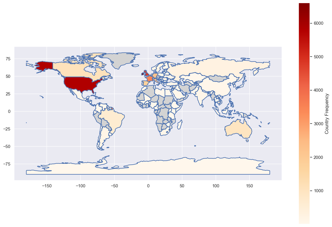
# There is a user from Antarctica!!
country_counts[country_counts['iso_a3'] == "ATA"]| CountryCode | Count | iso_a3 | |
|---|---|---|---|
| 130 | AQ | 1 | ATA |
Difference between Searching Date and Checkin Date
plt.figure(figsize=(10, 6))

sns.kdeplot(user_search_data[user_search_data['type_order'] == 0]['day_diff'], bw_adjust=0.5, fill=True, label='Search')
sns.kdeplot(user_search_data[user_search_data['type_order'] == 1]['day_diff'], bw_adjust=0.5, fill=True, label='Inquiry')
sns.kdeplot(user_search_data[user_search_data['type_order'] == 2]['day_diff'], bw_adjust=0.5, fill=True, label='Accepted')
sns.kdeplot(user_search_data[user_search_data['type_order'] == 3]['day_diff'], bw_adjust=0.5, fill=True, label='Book')
plt.title('Distribution of the Difference between Searching Date and Checkin Date')
plt.xlabel('Days')
plt.ylabel('Density')
plt.legend()
plt.show()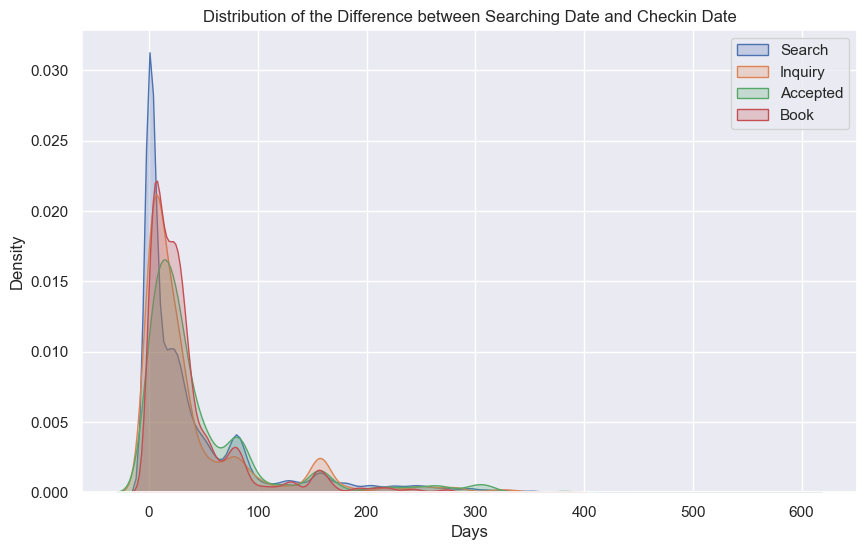
Number of Searches for Each Unique User
plt.figure(figsize=(10, 6))

sns.kdeplot(user_search_data[user_search_data['type_order'] == 0]['num_of_searches'], bw_adjust=0.5, fill=True, label='Search')
sns.kdeplot(user_search_data[user_search_data['type_order'] == 1]['num_of_searches'], bw_adjust=0.5, fill=True, label='Inquiry')
sns.kdeplot(user_search_data[user_search_data['type_order'] == 2]['num_of_searches'], bw_adjust=0.5, fill=True, label='Accepted')
sns.kdeplot(user_search_data[user_search_data['type_order'] == 3]['num_of_searches'], bw_adjust=0.5, fill=True, label='Book')
plt.title('Distribution of umber of Searches for Each Unique User')
plt.xlabel('Count')
plt.ylabel('Density')
plt.legend()
plt.show()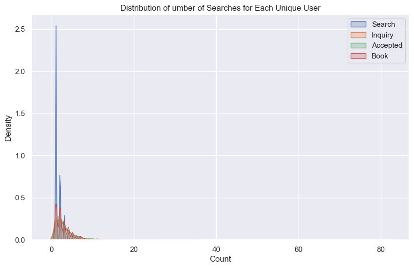
plt.figure(figsize=(10, 6))

sns.kdeplot(user_search_data[user_search_data['type_order'] == 0]['num_of_searches'], clip=(0,10), bw_adjust=0.2, fill=True, label='Search')
sns.kdeplot(user_search_data[user_search_data['type_order'] == 1]['num_of_searches'], clip=(0,10), bw_adjust=0.2, fill=True, label='Inquiry')
sns.kdeplot(user_search_data[user_search_data['type_order'] == 2]['num_of_searches'], clip=(0,10), bw_adjust=0.2, fill=True, label='Accepted')
sns.kdeplot(user_search_data[user_search_data['type_order'] == 3]['num_of_searches'], clip=(0,10), bw_adjust=0.2, fill=True, label='Book')
plt.title('Distribution of umber of Searches for Each Unique User')
plt.xlabel('Count')
plt.ylabel('Density')
plt.legend()
plt.show()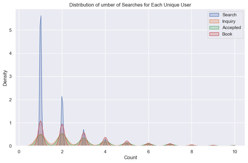
See here decided why to use median and tree model
fig, axes = plt.subplots(nrows=2, ncols=2, figsize=(12, 10))
fig.suptitle('Box Plots to Identify Outliers in Numerical Columns', fontsize=16)

num_cols = ['n_searches', 'n_nights', 'filter_price_min', 'filter_price_max']
for ax, col in zip(axes.flatten(), num_cols):
    df_s.boxplot(column=col, ax=ax)
    ax.set_title(col)

plt.tight_layout(rect=[0, 0.03, 1, 0.95])
plt.show()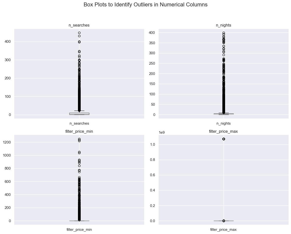
Model Training
We first use XGBoost, cross validation to find the best parameter.
X = user_search_data.copy().drop(['id_user'], axis=1)
y = X.pop("type_order")
X_train, X_valid, y_train, y_valid = train_test_split(X,y,test_size=0.2)
def objective(trial):
params = {
'n_estimators': trial.suggest_int('n_estimators', 500, 2000),
'learning_rate': trial.suggest_float('learning_rate', 1e-4, 0.1),
'max_depth': trial.suggest_int('max_depth', 5, 40),
'min_child_weight': trial.suggest_float('min_child_weight', 0.5, 4),
'subsample': trial.suggest_float('subsample', 0.2, 1),
'colsample_bytree': trial.suggest_float('colsample_bytree', 0.2, 1),
'lambda': trial.suggest_float('lambda', 1e-8, 1.0), # L2 regularization
'alpha': trial.suggest_float('alpha', 1e-8, 1.0), # L1 regularization
'use_label_encoder': False, # Avoid a deprecation warning
}
xgb_model = XGBClassifier(**params, eval_metric='mlogloss', verbosity=0)
cv = cross_val_score(xgb_model, X, y, cv=4, scoring='accuracy').mean()
return cv
study = optuna.create_study(direction='maximize')
study.optimize(objective, n_trials=100, timeout=1800, show_progress_bar=True)
print('Best trial:')
trial = study.best_trial
print('Value: ', trial.value)
print('Params: ')
for key, value in trial.params.items():
print(f' {key}: {value}')[I 2024-04-13 20:48:27,128] A new study created in memory with name: no-name-c61da181-f6f0-4406-a28e-2ca6ef57cfcc[I 2024-04-13 20:49:31,625] Trial 0 finished with value: 0.813813466274415 and parameters: {'n_estimators': 1337, 'learning_rate': 0.047229613231243694, 'max_depth': 18, 'min_child_weight': 1.5004360596379311, 'subsample': 0.48720956244704877, 'colsample_bytree': 0.24118622095320275, 'lambda': 0.5198374651782831, 'alpha': 0.6542260507192192}. Best is trial 0 with value: 0.813813466274415.
[I 2024-04-13 20:51:45,982] Trial 1 finished with value: 0.8203711033583511 and parameters: {'n_estimators': 1624, 'learning_rate': 0.006477410403064766, 'max_depth': 27, 'min_child_weight': 1.9391492954946157, 'subsample': 0.26393362218029454, 'colsample_bytree': 0.958667550622444, 'lambda': 0.7275514654420072, 'alpha': 0.24795684861624576}. Best is trial 1 with value: 0.8203711033583511.
[I 2024-04-13 20:54:00,094] Trial 2 finished with value: 0.8025263915728882 and parameters: {'n_estimators': 1822, 'learning_rate': 0.04379408103268792, 'max_depth': 19, 'min_child_weight': 3.2587794436607522, 'subsample': 0.6397393146522905, 'colsample_bytree': 0.9778316529309103, 'lambda': 0.5242213883065793, 'alpha': 0.640957442042659}. Best is trial 1 with value: 0.8203711033583511.
[I 2024-04-13 20:55:31,997] Trial 3 finished with value: 0.7984413988023544 and parameters: {'n_estimators': 1625, 'learning_rate': 0.09525925387395676, 'max_depth': 20, 'min_child_weight': 3.8200242269078672, 'subsample': 0.5442124924293351, 'colsample_bytree': 0.657405813353553, 'lambda': 0.1247179047579049, 'alpha': 0.8382256793834322}. Best is trial 1 with value: 0.8203711033583511.
[I 2024-04-13 20:57:10,276] Trial 4 finished with value: 0.8130075000281931 and parameters: {'n_estimators': 1280, 'learning_rate': 0.01682254047988452, 'max_depth': 24, 'min_child_weight': 2.2456629893841953, 'subsample': 0.4245461662781999, 'colsample_bytree': 0.9693097176818797, 'lambda': 0.6012631974370846, 'alpha': 0.5096914842848129}. Best is trial 1 with value: 0.8203711033583511.
[I 2024-04-13 20:59:07,689] Trial 5 finished with value: 0.8002688587759212 and parameters: {'n_estimators': 1859, 'learning_rate': 0.061011727815679616, 'max_depth': 40, 'min_child_weight': 2.5507746123075745, 'subsample': 0.2686234674222428, 'colsample_bytree': 0.9036252567648639, 'lambda': 0.40555021926099183, 'alpha': 0.7614547968380192}. Best is trial 1 with value: 0.8203711033583511.
[I 2024-04-13 20:59:58,396] Trial 6 finished with value: 0.824509663137006 and parameters: {'n_estimators': 552, 'learning_rate': 0.009244780950413032, 'max_depth': 21, 'min_child_weight': 1.1776475763509335, 'subsample': 0.5787484399490634, 'colsample_bytree': 0.6717104435517728, 'lambda': 0.27308200188135845, 'alpha': 0.6604682731983871}. Best is trial 6 with value: 0.824509663137006.
[I 2024-04-13 21:00:50,344] Trial 7 finished with value: 0.8154797399314824 and parameters: {'n_estimators': 1133, 'learning_rate': 0.07299712057147484, 'max_depth': 13, 'min_child_weight': 1.3292628334912076, 'subsample': 0.8438719229660459, 'colsample_bytree': 0.2002516250948327, 'lambda': 0.8198157691830962, 'alpha': 0.8928324142818284}. Best is trial 6 with value: 0.824509663137006.
[I 2024-04-13 21:03:00,417] Trial 8 finished with value: 0.8154260458230398 and parameters: {'n_estimators': 1534, 'learning_rate': 0.017041429123773714, 'max_depth': 30, 'min_child_weight': 1.722301834175352, 'subsample': 0.656351410385265, 'colsample_bytree': 0.5333034234046892, 'lambda': 0.10003377531260546, 'alpha': 0.5853008152606514}. Best is trial 6 with value: 0.824509663137006.
[I 2024-04-13 21:03:43,984] Trial 9 finished with value: 0.8259607790593393 and parameters: {'n_estimators': 686, 'learning_rate': 0.0009626545964325102, 'max_depth': 15, 'min_child_weight': 0.8950946674929849, 'subsample': 0.653682987578901, 'colsample_bytree': 0.9653556818615103, 'lambda': 0.9981782746720972, 'alpha': 0.8084151115559389}. Best is trial 9 with value: 0.8259607790593393.
[I 2024-04-13 21:03:58,621] Trial 10 finished with value: 0.826068352149419 and parameters: {'n_estimators': 534, 'learning_rate': 0.029566664080238888, 'max_depth': 6, 'min_child_weight': 0.5493692401340649, 'subsample': 0.9582245810596254, 'colsample_bytree': 0.7785256985419187, 'lambda': 0.9163152035026848, 'alpha': 0.26196592563605225}. Best is trial 10 with value: 0.826068352149419.
[I 2024-04-13 21:04:11,245] Trial 11 finished with value: 0.8261220924761601 and parameters: {'n_estimators': 530, 'learning_rate': 0.030412496626778224, 'max_depth': 5, 'min_child_weight': 0.5009248161992941, 'subsample': 0.9670656084409862, 'colsample_bytree': 0.7708009548973506, 'lambda': 0.9982146279800529, 'alpha': 0.2380032301548375}. Best is trial 11 with value: 0.8261220924761601.
[I 2024-04-13 21:04:31,200] Trial 12 finished with value: 0.8250471819501645 and parameters: {'n_estimators': 867, 'learning_rate': 0.032734589881235905, 'max_depth': 5, 'min_child_weight': 0.5352160584504654, 'subsample': 0.9953504502364621, 'colsample_bytree': 0.7988319275869853, 'lambda': 0.9832896170125175, 'alpha': 0.21798153039974583}. Best is trial 11 with value: 0.8261220924761601.
[I 2024-04-13 21:04:50,877] Trial 13 finished with value: 0.8249934416234233 and parameters: {'n_estimators': 871, 'learning_rate': 0.03333523971613389, 'max_depth': 5, 'min_child_weight': 0.5819147172295058, 'subsample': 0.9592633112246078, 'colsample_bytree': 0.807339787548702, 'lambda': 0.8160869169231629, 'alpha': 0.022940498384892316}. Best is trial 11 with value: 0.8261220924761601.
[I 2024-04-13 21:05:17,692] Trial 14 finished with value: 0.8234884698286022 and parameters: {'n_estimators': 551, 'learning_rate': 0.03023121180316528, 'max_depth': 10, 'min_child_weight': 1.0492797175238322, 'subsample': 0.8058336751399967, 'colsample_bytree': 0.5322391452470353, 'lambda': 0.8713844462828828, 'alpha': 0.3076091161667134}. Best is trial 11 with value: 0.8261220924761601.
[I 2024-04-13 21:05:58,489] Trial 15 finished with value: 0.8082776117821906 and parameters: {'n_estimators': 934, 'learning_rate': 0.06462866610737526, 'max_depth': 9, 'min_child_weight': 2.732941476903637, 'subsample': 0.8279724926318875, 'colsample_bytree': 0.7560034708481365, 'lambda': 0.6708791399556301, 'alpha': 0.38989071871013525}. Best is trial 11 with value: 0.8261220924761601.
[I 2024-04-13 21:06:26,387] Trial 16 finished with value: 0.8241871980674096 and parameters: {'n_estimators': 695, 'learning_rate': 0.023893451508534832, 'max_depth': 9, 'min_child_weight': 0.8047267398489057, 'subsample': 0.8865787380701572, 'colsample_bytree': 0.4895347101413101, 'lambda': 0.8909494046771829, 'alpha': 0.05934635947850925}. Best is trial 11 with value: 0.8261220924761601.
[I 2024-04-13 21:07:40,460] Trial 17 finished with value: 0.8135986205131969 and parameters: {'n_estimators': 1037, 'learning_rate': 0.04424298317396684, 'max_depth': 37, 'min_child_weight': 0.5557605600982021, 'subsample': 0.7473014965520811, 'colsample_bytree': 0.34538123082588207, 'lambda': 0.7451447802738025, 'alpha': 0.14116553608857246}. Best is trial 11 with value: 0.8261220924761601.
[I 2024-04-13 21:08:25,855] Trial 18 finished with value: 0.8100512736561429 and parameters: {'n_estimators': 667, 'learning_rate': 0.056354576952966924, 'max_depth': 14, 'min_child_weight': 1.9175694242757688, 'subsample': 0.9266279983348323, 'colsample_bytree': 0.7124872198711556, 'lambda': 0.39553012835088786, 'alpha': 0.3748087445659024}. Best is trial 11 with value: 0.8261220924761601.
[I 2024-04-13 21:08:39,630] Trial 19 finished with value: 0.8216072579737196 and parameters: {'n_estimators': 505, 'learning_rate': 0.07807390321146618, 'max_depth': 5, 'min_child_weight': 1.447761828581032, 'subsample': 0.7411336604528174, 'colsample_bytree': 0.8482182716247123, 'lambda': 0.9387511733773851, 'alpha': 0.4393780417462038}. Best is trial 11 with value: 0.8261220924761601.
[I 2024-04-13 21:09:33,807] Trial 20 finished with value: 0.8134372724326521 and parameters: {'n_estimators': 772, 'learning_rate': 0.036428337416606144, 'max_depth': 33, 'min_child_weight': 2.986317642055114, 'subsample': 0.36216400097035273, 'colsample_bytree': 0.6045081342768153, 'lambda': 0.6542072354177585, 'alpha': 0.11405944484416197}. Best is trial 11 with value: 0.8261220924761601.
[I 2024-04-13 21:10:35,815] Trial 21 finished with value: 0.8262295384659185 and parameters: {'n_estimators': 678, 'learning_rate': 0.00027262230602636075, 'max_depth': 15, 'min_child_weight': 1.0116302454830888, 'subsample': 0.7237819360653299, 'colsample_bytree': 0.8696735760725043, 'lambda': 0.9979845742208219, 'alpha': 0.19502713141165656}. Best is trial 21 with value: 0.8262295384659185.
[I 2024-04-13 21:11:11,389] Trial 22 finished with value: 0.8244022171472476 and parameters: {'n_estimators': 510, 'learning_rate': 0.020788198953459194, 'max_depth': 11, 'min_child_weight': 0.8780630344106966, 'subsample': 0.7548131898342476, 'colsample_bytree': 0.8599940681890501, 'lambda': 0.907393538757365, 'alpha': 0.1913947587815238}. Best is trial 21 with value: 0.8262295384659185.
[I 2024-04-13 21:11:40,793] Trial 23 finished with value: 0.8266596343984679 and parameters: {'n_estimators': 778, 'learning_rate': 0.009306603424580433, 'max_depth': 8, 'min_child_weight': 1.06465509758388, 'subsample': 0.9072207944572264, 'colsample_bytree': 0.7658441822251906, 'lambda': 0.783959485397532, 'alpha': 0.30582332667893436}. Best is trial 23 with value: 0.8266596343984679.
[I 2024-04-13 21:12:58,877] Trial 24 finished with value: 0.8247784340981599 and parameters: {'n_estimators': 786, 'learning_rate': 0.000899010873623342, 'max_depth': 16, 'min_child_weight': 1.1711545565925352, 'subsample': 0.8626388874125682, 'colsample_bytree': 0.8746125769801567, 'lambda': 0.7905707125061482, 'alpha': 0.3379222447871222}. Best is trial 23 with value: 0.8266596343984679.
[I 2024-04-13 21:13:44,056] Trial 25 finished with value: 0.824939701296682 and parameters: {'n_estimators': 1023, 'learning_rate': 0.011620423872540342, 'max_depth': 8, 'min_child_weight': 1.5731654000013582, 'subsample': 0.8888144477272626, 'colsample_bytree': 0.7354268068603133, 'lambda': 0.999866701875694, 'alpha': 0.4629631308606137}. Best is trial 23 with value: 0.8266596343984679.
[I 2024-04-13 21:14:31,938] Trial 26 finished with value: 0.8242947133846159 and parameters: {'n_estimators': 635, 'learning_rate': 0.011948647446816604, 'max_depth': 12, 'min_child_weight': 0.8917237020680562, 'subsample': 0.7069706700284674, 'colsample_bytree': 0.6806805770029137, 'lambda': 0.8420137513945466, 'alpha': 0.1579317861953075}. Best is trial 23 with value: 0.8266596343984679.
[I 2024-04-13 21:15:51,394] Trial 27 finished with value: 0.8145124024955662 and parameters: {'n_estimators': 814, 'learning_rate': 0.023518283467701503, 'max_depth': 17, 'min_child_weight': 2.1531941423259515, 'subsample': 0.9951758044390351, 'colsample_bytree': 0.9101319895013484, 'lambda': 0.7454106511469829, 'alpha': 0.29914243167348653}. Best is trial 23 with value: 0.8266596343984679.
[I 2024-04-13 21:16:49,961] Trial 28 finished with value: 0.8274658201816083 and parameters: {'n_estimators': 1171, 'learning_rate': 0.004693099965535389, 'max_depth': 8, 'min_child_weight': 1.2895967986038595, 'subsample': 0.7804638105059425, 'colsample_bytree': 0.6081963765934802, 'lambda': 0.9255099991762942, 'alpha': 0.06406101879012513}. Best is trial 28 with value: 0.8274658201816083.
[I 2024-04-13 21:18:28,451] Trial 29 finished with value: 0.8258532175238343 and parameters: {'n_estimators': 1444, 'learning_rate': 0.0038715750889392595, 'max_depth': 13, 'min_child_weight': 1.697845224896466, 'subsample': 0.7983637803530047, 'colsample_bytree': 0.4022918223666994, 'lambda': 0.6511410294605691, 'alpha': 0.08047711382215175}. Best is trial 28 with value: 0.8274658201816083.
Best trial:
Value: 0.8274658201816083
Params:
n_estimators: 1171
learning_rate: 0.004693099965535389
max_depth: 8
min_child_weight: 1.2895967986038595
subsample: 0.7804638105059425
colsample_bytree: 0.6081963765934802
lambda: 0.9255099991762942
alpha: 0.06406101879012513xgb_classifier = XGBClassifier()
xgb_classifier.fit(X_train, y_train)
y_pred = xgb_classifier.predict(X_valid)
xgb_accuracy_score = accuracy_score(y_valid, y_pred)
print("XGBClassifier Accuracy:", xgb_accuracy_score)XGBClassifier Accuracy: 0.8212846009137329Comparing with other models, we use the combined model called voting classifier to identify the stage of people.
rf_classifier = RandomForestClassifier()
rf_classifier.fit(X_train, y_train)
rf_y_pred = rf_classifier.predict(X_valid)
rf_accuracy_score = accuracy_score(y_valid, rf_y_pred)
rf_accuracy_score0.8105348024724537mlp_classifier = MLPClassifier()
mlp_classifier.fit(X_train, y_train)
mlp_y_pred = mlp_classifier.predict(X_valid)
mlp_accuracy_score = accuracy_score(y_valid, mlp_y_pred)
mlp_accuracy_score0.806503628056974svm_classifier = SVC(probability=True)
svm_classifier.fit(X_train, y_train)
svm_y_pred = svm_classifier.predict(X_valid)
svm_accuracy_score = accuracy_score(y_valid, svm_y_pred)
svm_accuracy_score0.8210158559527009Voting Classifier
classifiers = [('random_forest', rf_classifier),
    ('svm', svm_classifier),
    ('mlp', mlp_classifier),
    ('xgb', xgb_classifier)
]

voting_clf = VotingClassifier(estimators=classifiers, voting='hard')
voting_clf.fit(X_train, y_train)
voting_pred = voting_clf.predict(X_valid)
voting_accuracy_score = accuracy_score(y_valid, voting_pred)
voting_accuracy_score0.8237033055630207xgb_classifier.feature_importances_array([0.03214042, 0.02455774, 0.02288991, 0.01597637, 0.0157053 ,
0.01522262, 0.01760654, 0.01486355, 0.01796535, 0.0191166 ,
0. , 0.01155449, 0. , 0. , 0. ,
0.01604011, 0.01683889, 0.01560377, 0. , 0. ,
0. , 0. , 0.01549766, 0. , 0.01013466,
0.02900742, 0. , 0. , 0.01473845, 0.00728089,
0.0157551 , 0.01849182, 0. , 0. , 0.01439588,
0.00661679, 0. , 0. , 0. , 0.01467162,
0.01698269, 0.01810054, 0. , 0. , 0. ,
0. , 0.00872591, 0.0160712 , 0. , 0. ,
0.01640791, 0.01694654, 0.01688639, 0. , 0. ,
0. , 0. , 0. , 0.0136373 , 0. ,
0.01868004, 0.01573102, 0.01299768, 0. , 0.03188633,
0.01033509, 0. , 0.01145769, 0. , 0. ,
0.01650339, 0. , 0.00598313, 0.00983884, 0. ,
0.01450301, 0. , 0. , 0. , 0.00576115,
0. , 0. , 0.00706745, 0.01864195, 0. ,
0. , 0. , 0. , 0. , 0. ,
0. , 0. , 0. , 0. , 0. ,
0.00629945, 0. , 0. , 0.01314489, 0.01169234,
0. , 0. , 0. , 0.01755105, 0.01236612,
0. , 0.01578866, 0. , 0. , 0.00903834,
0. , 0.01211253, 0. , 0.01390858, 0. ,
0. , 0.01319115, 0.01226211, 0.01494829, 0.01316986,
0.01216134, 0.01945747, 0.00908214, 0.00818385, 0. ,
0. , 0. , 0.00898265, 0. , 0.01442079,
0.01242575, 0. , 0.01064345, 0. , 0.01584867,
0. , 0. , 0. , 0. , 0.01750329,
0. ], dtype=float32)Decision Boundaries
That is a really complex model
# Extract the two features and the target variable
X = user_search_data[['num_of_searches', 'day_diff']]
y = user_search_data['type_order']

X_train, X_test, y_train, y_test = train_test_split(X, y, test_size=0.2, random_state=42)

classifier = XGBClassifier()
classifier.fit(X_train, y_train)

# Create a mesh to plot in
x_min, x_max = X['num_of_searches'].min() - 1, X['num_of_searches'].max() + 1
y_min, y_max = X['day_diff'].min() - 1, X['day_diff'].max() + 1
xx, yy = np.meshgrid(np.arange(x_min, x_max, 0.1),
                     np.arange(y_min, y_max, 0.1))

# Predict on the mesh
Z = classifier.predict(np.c_[xx.ravel(), yy.ravel()])
Z = Z.reshape(xx.shape)

plt.figure(figsize=(10, 6))
plt.contourf(xx, yy, Z, alpha=0.8, cmap=ListedColormap(['#FFAAAA', '#AAAAFF']))
plt.xlabel('num_of_searches')
plt.ylabel('day_diff')
plt.xlim(xx.min(), xx.max())
plt.ylim(yy.min(), yy.max())
plt.title('Decision Boundary with XGBoost')
plt.show()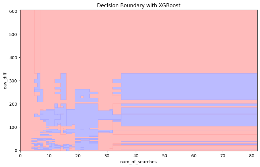
Conclusion
Marketing campaign should be performed around 25 days before the busy season for traveling
Encourage users to do more searching
Our model can predict the user’s “drop out” stage, therefore we can make accurate action to avoid this.
 Created in